
What if the scoreboard is lying?
Expected goals, or xG, fixes that by putting a probability on every shot and adding them up to show how dangerous a team or player really is.
It strips out luck and bounces to reveal the process behind goals.
That matters for coaches, scouts, parents, and players because xG shows who’s creating real chances, which systems work, and when hot streaks will fade.
This guide explains how xG is calculated, what to trust, and how to use it for better hockey decisions.
Core Explanation of Expected Goals (xG) in Hockey

Expected goals (xG) assigns a probability to each shot based on how likely it is to score. The system looks at thousands of historical shots to figure out that a wrist shot from the slot beats a slapshot from the blue line pretty much every time. You add up all those shot probabilities from a game, and that’s your xG total.
This beats traditional stats because it separates how many shots you took from how dangerous they actually were. A team can launch thirty shots and still create less real danger than an opponent who only gets twelve clean looks. Goals are messy. Bounces happen, guys get hot, goalies have bad nights. Expected goals cuts through that noise and shows you what was actually happening before luck showed up.
Hockey people use xG to spot which players create dangerous chances, which teams run systems that actually work, and which results are going to stick around. When a team outscores its xG by twenty goals in October, most of that gap vanishes by January. Expected goals reveals the process driving wins and losses.
- Shot-level probability – Each shot gets an xG value between 0 and 1 based on how often that type of shot goes in
- Quality over volume – Three slot chances can be worth more than fifteen shots from the outside
- Team and player totals – Add up shot-level xG and you get team xG for/against and player xG per 60 minutes
- Sustainability check – Teams with strong xG advantages usually keep winning, even when goals aren’t falling yet
- Context for outcomes – A goalie allowing fifteen goals on eighteen xG faced way different work than one allowing fifteen on twelve xG
How Expected Goals Are Calculated

Expected goals models study historical shot data to build a prediction system. Most models start with basic play-by-play info and add tracking details when they can get them. The point is to estimate how often a shot from a specific spot and situation actually goes in.
Two common methods are logistic regression and gradient-boosted trees. Logistic regression gives you clear numbers and stays stable. Gradient-boosted methods like XGBoost and LightGBM usually predict better because they catch patterns that aren’t straight lines. Both spit out a probability that gets assigned to each new shot.
The factors that matter most:
- Shot distance – Shots from ten feet score way more than shots from forty feet. Distance is the biggest piece.
- Shot angle – Sharp-angle attempts from the goal line don’t go in as much as centered shots from the same spot
- Shot type – Wrist shots, slap shots, deflections, and one-timers all convert at different rates
- Rebound status – Shots right after a save or block carry higher danger
- Pre-shot movement – Rush chances, odd-man breaks, and cross-ice passes pump up xG
- Traffic and screens – Shots through bodies or with a screened goalie jump in probability
- Manpower state – Power-play shots convert more than even-strength, so models often split 5v5, PP, and PK
Public xG models use league play-by-play data with shot coordinates, event types, and basic context. Team models add optical tracking, shot speed, goalie position, and exact pass timing. Better data means sharper predictions, but even basic models work when they’re built right.
Applying xG to Evaluate Players
Expected goals separates creating chances from finishing them. A player piling up individual xG is generating dangerous shots no matter how many actually cross the line. A player scoring well above their xG shows elite finishing or a hot streak, and you watch to see which one it is.
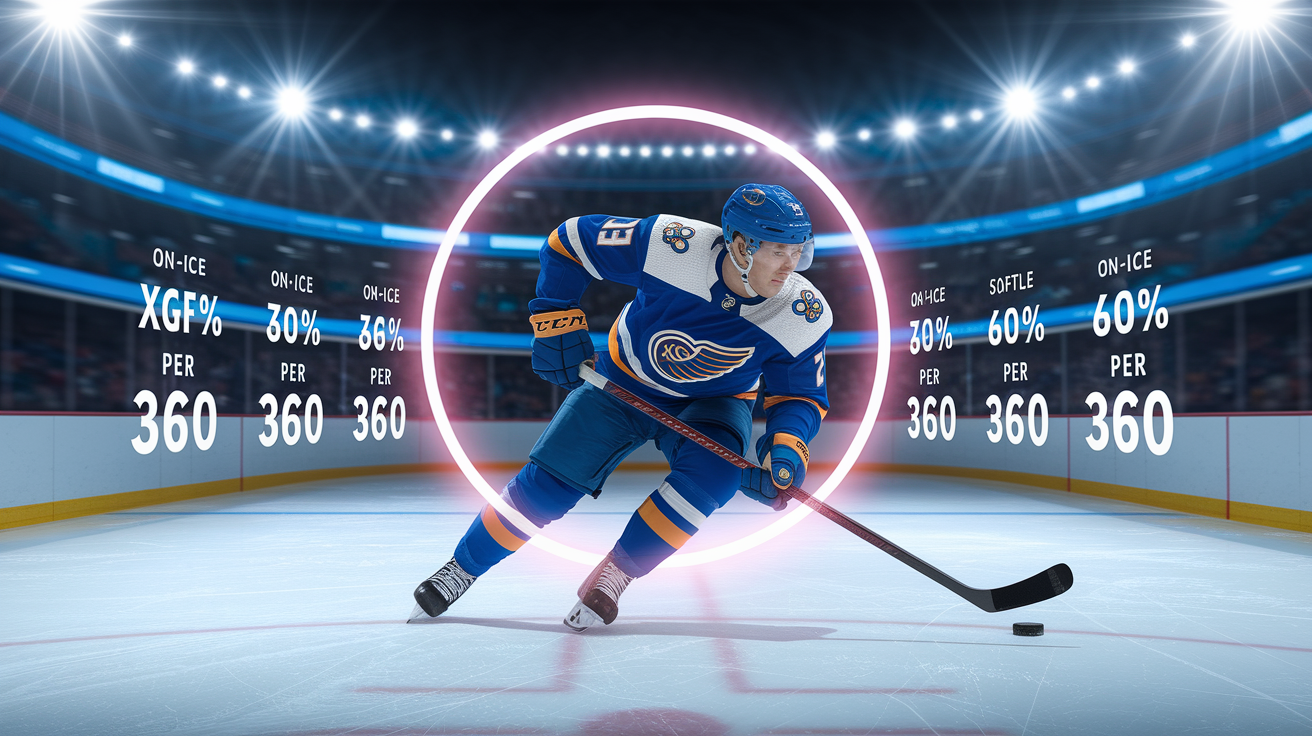
Individual xG per sixty minutes normalizes for ice time and shows offensive output without linemates or power-play inflation getting in the way. On-ice xG captures all shots while a player’s out there, giving you the full offensive and defensive picture. A winger with strong on-ice xGF% drives play the right direction even if their personal goal count looks quiet.
Finding overperformers and underperformers takes sample size. A player with 250 shots and twelve expected goals who scores eighteen sits six goals above xG. That could be skill or variance. Wait for another 200 shots before you decide. Beating xG over 400 shots suggests real finishing ability. Running below xG over the same stretch points to bad luck, poor shot picks, or needing to adjust release points.
Team-Level Insights from xG

Team xG differential (xGF minus xGA per game) lines up tight with winning percentage and playoff success. A team pumping out 3.5 xG per game while giving up 2.8 xG projects more wins than a team sitting at 2.9 xGF and 3.2 xGA, even when short-term results say something different.
Systems built around puck possession in dangerous spots, active net-front presence, and quick cross-ice passes show up in xG before they show up in standings. Defensive setups that kill slot access and shut down passing lanes cut xGA. When a team’s actual goals blow past xG over twenty games, expect things to even out unless their shooting or goaltending is genuinely elite.
| Team Metric | Meaning | Insight Provided |
|---|---|---|
| xGF/60 | Expected goals for per 60 minutes | How fast you create dangerous chances, sustainable scoring potential |
| xGA/60 | Expected goals against per 60 minutes | Shot quality you’re giving up, where your structure breaks down or holds |
| xG Differential | xGF minus xGA per game | Real team quality, tells you more about future wins than current record |
| xGF% | Team xGF divided by total xG (for + against) | Share of expected goals in all situations, puck control and territorial edge |
Using xG to Evaluate Goalies

Goalie evaluation with expected goals starts with expected goals against (xGA), which is just the sum of xG from every shot they faced. Goals Saved Above Expected (GSAx) is xGA minus actual goals allowed. A goalie facing 180 xGA over a season who allows 165 goals posts +15 GSAx, meaning he saved fifteen more than the model predicted.
GSAx per sixty minutes accounts for workload. A goalie with +0.10 GSAx/60 over 2,000 minutes shows steady performance above expected shot quality. Small samples are noisy, so don’t trust any GSAx read based on fewer than 1,000 minutes. Goalies facing high xGA work behind weaker structures or see more high-danger looks, and raw save percentage doesn’t tell that story. A goalie with .910 who faced tough shots may have actually outperformed someone with .915 who got easier work.
Interpreting Overperformance and Underperformance

Overperformance is when actual goals blow past expected goals. A team scoring 315 on 280 xG sits +35 above expectation. Some of that is elite finishing. Most is variance that disappears over the next fifty games. Analysts flag anything beyond ten goals and track whether it holds or fades.
Sustained overperformance across a full season with stable xG inputs says the team’s got high-skill finishers or a system creating better looks than standard models catch. If the xG differential itself is positive and big, the team’s legit. If actual goals are way ahead of xG but the underlying differential is negative, expect the record to tank when finishing normalizes.
Underperformance shows up as actual goals way below xG. A player with fifteen xG and nine goals through forty games is running cold. Before calling them a bad finisher, check shot selection, release consistency, and whether the model accounts for shooter identity. When a whole team underperforms, it usually points to a dead power play, a struggling top line, or a stretch of rough goaltending killing goals for. Track it across twenty to thirty games and combine xG with video to separate skill issues from slumps.
Data Sources and Tools for xG

Public hockey sites give you xG models, dashboards, and downloadable data covering every NHL game. Each platform uses slightly different features and methods, so xG values for the same shot can shift a few percentage points between sources.
- Evolving-Hockey – Player cards, team reports, xG totals per game and per sixty, GSAx for goalies, historical trends. Models include distance, angle, type, rush context, rebound flags.
- MoneyPuck – xG heatmaps, shot-quality charts, game predictions. Adds pre-shot movement and pass sequences.
- Natural Stat Trick – Situational xG splits (5v5, power play, penalty kill), zone-start adjustments, score-state filters. Fast lookups, custom queries.
- NHL Edge tracking data – League puck and player tracking with shot speed and location. Some Edge-based xG models are proprietary, but select stats show up on NHL.com.
Practical Examples Using NHL Data

During 2021–2022, the Florida Panthers led the league in goals and sat near the top in xGF. Their xG differential stayed positive all year, signaling real offensive firepower instead of a shooting-percentage fluke. When actual goal totals dipped slightly in the second half, the underlying xG stayed strong, and analysts correctly called continued success into the playoffs.
A forward finishing with twenty-five goals on eighteen xG is clearly overperforming. Scouts and front offices looking at that player for a contract extension will check shot volume, xG per sixty, linemate quality, and whether the finishing gap held across multiple seasons. If the player beats xG by small margins over 600+ shots, the skill’s real. If the gap popped up in one fifty-game run, regression’s coming and the contract offer drops.
Team systems work gets measured with xG too. A club switching from dump-and-chase to controlled entries typically sees xGF rise before goal totals follow. Coaching staffs use rolling ten-game xG differentials to check whether new line combos or defensive pairings actually improve shot quality. When xGA drops after a scheme tweak but actual goals allowed stay flat, the change is working and results will catch up once goaltending variance smooths out.
Limitations and Common Misinterpretations of xG

Expected goals models don’t perfectly account for individual shooting talent unless shooter identity gets baked in as a feature, and most public models skip it to avoid overfitting. Two players taking identical shots from the same spot get the same xG value even if one’s got a way better release. This means xG measures opportunity quality, not outcome certainty.
Different models spit out different xG totals for the same game because feature sets and training data vary. One might give a team 2.8 xG while another says 3.1. Team rank order and trends usually line up, but absolute values shift. Don’t mix outputs from multiple models in a single calculation, and always note the source.
Small samples lie. A ten-game stretch where a player scores eight goals on four xG looks incredible but tells you nothing about skill. Variance owns short windows. Pair xG with video, context about opponent strength, score effects (teams protecting leads take fewer dangerous shots), and other metrics like zone entries, pass completion, and defensive impacts. Expected goals is one tool, not the whole answer.
Workflow for Integrating xG into Hockey Analysis
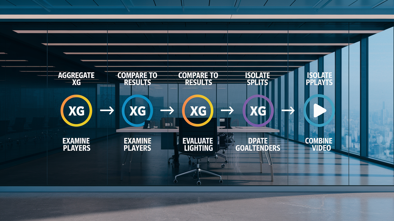
Getting expected goals into your regular work starts with clean shot-level data from a solid public source or proprietary tracking system. Grab game logs with xG per shot, player on-ice details, and situational context like score state and manpower.
- Aggregate xG totals – Add up shot-level xG to get team xGF and xGA per game, per sixty, across custom date ranges
- Compare to actual results – Plot xG differential against actual goal differential to spot overperforming and underperforming stretches
- Isolate situational splits – Break out even-strength, power-play, and penalty-kill xG to see where a team or player shines or struggles
- Examine individual players – Check xG/60 and on-ice xGF% for each skater, flag anyone with big gaps between xG and goals
- Evaluate goalies – Calculate GSAx and GSAx/60 to measure performance versus shot quality faced
- Combine with video and context – Use xG trends to guide film sessions, zero in on plays that created high xG or gave up dangerous chances. Fold findings into reports, lineup calls, and opponent scouting.
Final Words
When you’re staring at a game’s shot map and wondering which chances mattered, xG gives a clearer answer. What it measures and why it matters was the first stop in this post.
We then walked through how xG is calculated, using it for player, team, and goalie evaluation, real NHL examples, common limits, public data sources, and a practical workflow you can use.
Use this guide to using expected goals (xG) in hockey analysis as your next checklist. Start applying xG on the next review and you’ll make smarter calls faster.
FAQ
Q: How are expected goals (xG) calculated in hockey?
A: Expected goals (xG) are calculated by fitting models on thousands of past NHL shots to assign each shot a scoring probability based on distance, angle, shot type, rebounds, pre-shot movement, screens, and pressure.
Q: What is expected goals against (xGA)?
A: Expected goals against (xGA) is the sum of scoring probabilities for shots a team or goalie faces, showing the quality of chances allowed and helping separate goalie performance from team defense.
Q: What is the xG strategy?
A: An xG strategy uses expected goals to drive decisions: identify where to create higher-quality chances, fix defensive holes, evaluate shooters and goalies, and guide lineup or tactical adjustments.